The logistic map

History

The logistic map is a mathematical model that is used to simulate the evolution of an animal population.
It's a simple equation that looks like that:

		x(t+1) = r * x(t) * (1 - x(t))

Where:

x(t) is the current population that can go between 0 and 1.
x(t+1) is the poulation at the next time step. Let's say the next year.
r is a "fertility rate". Its value must stay between 0 and 4 to keep the population between 0 and 1.

The first part of this equation "r * x(t)" is easy to understand: The current population mutiplied by the fertility
rate gives the new population.
The second part "(1 - x(t))" is a bit more difficult to explain. It represents a "death ratio" due to the food
limitation and the interactions between the animals.

Although this equation seems simple its evolution is quite complex when r changes.
And it displays a chaotic behavior for the highest values of r.

It does not only models populations but it's also used in economics or neural networks.
Stanislaw Ulam and John von Neumann wanted to use it as a random number generator.
And this equation is also linked to the Mandelbrot set as you can see it in a video in the links section.

Various behaviours

We'll write a simple program to display the evolution of an initial population of 0.5 with a given value of r.
Each value we will compute with the equation will be separated by 10 pixels along the x axis.

		#define WIDTH   10

We define our value for "r":

		float r = 0.95f;

Then in the main loop we clear the screen and initialize the starting x to 0.5

		while (sys.isQuitRequested() == false)
		{
			gfx.clearScreen(Color(0, 0, 0, SDL_ALPHA_OPAQUE));
			float x = 0.5f;

We loop along the screen width 10 pixels by 10 pixels:

			for (int t = 0; t < SCREEN_WIDTH - 1; t += WIDTH)
			{

We store the current value of x, and we compute the new value with the equation

				float oldX = x;
				x = r * x * (1 - x);

We multiply these values by the screen height to get a pixel y coordinate.

				int oldY = (1 - oldX) * (SCREEN_HEIGHT - 1);
				int y    = (1 - x)    * (SCREEN_HEIGHT - 1);

And finally we draw a line between these 2 points:

				gfx.line(t, oldY, t + WIDTH, y, Color(255, 255, 255));
			}

		Download source code
		Download executable for Windows

Now let's see what happens with various values of the fertility rate.
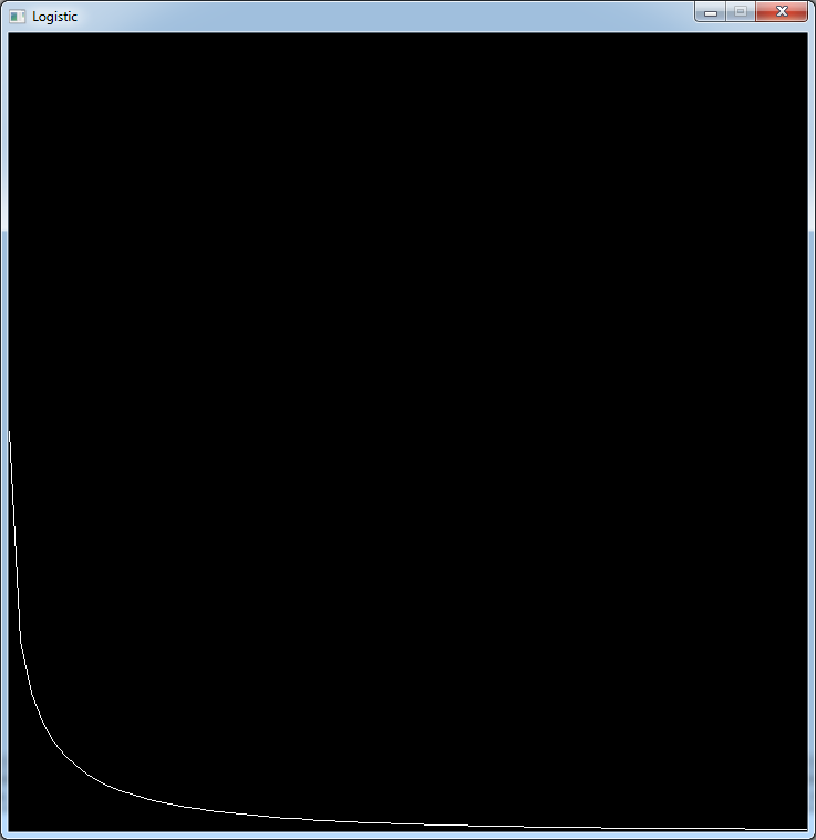
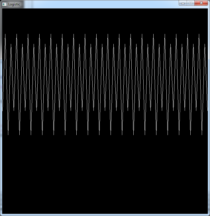
When r is between 0 and 1, the population quickly dies.
Here is the result for r = 0.95:

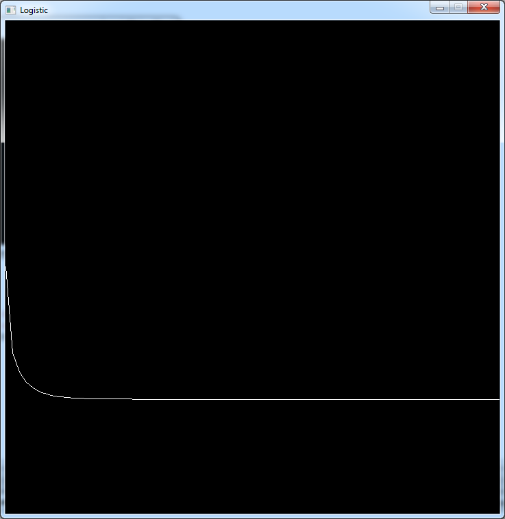
Between 1 and 2 the population stabilizes to a value below its starting point.
Here for r =1.3:

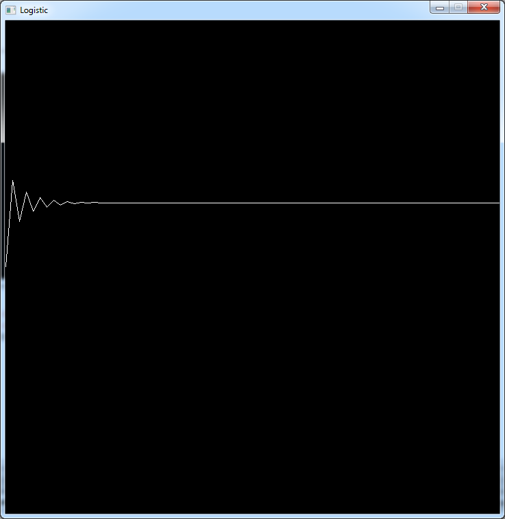
Between 2 and 3.1 the population oscillates a litte bit then stabilizes to a value higher than the starting
point.
For r = 2.7:

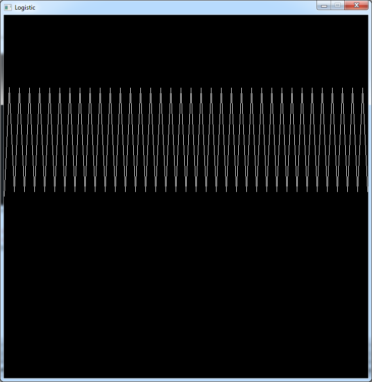
Between 3 and 3.44 the population oscillates between 2 values
For r = 3.2:

Between 3.44 and 3.54 the population oscillates between 4 values
For r = 3.5:

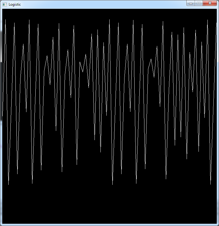
Above 3.54 the curve seems to be more and more random
For r = 3.8:

We can make a small modification to the code to animate the value of r and understand more easily what happens.
At the beginning we initialize it with 0:

		float r = 0.0f;

Then at the end of the main loop we will add a few lines to increase it slowly and set it back to 0 when it gets
over 4:

		sys.wait(16);
		r += 0.002f;

		if (r > 4.0f)
			r = 0.0f;

		Download source code
		Download executable for Windows

You can see the result on my youtube channel. See the link at the end of this article.

The bifurcation diagram

Another way to visualize the stable points of this system is to draw a diagram where r varies along the x axis.
For each of these r values we will draw a point where the population is after N iterations.
Where N is a big value like 10000.
But as the system may oscillate we will also draw a point after N+1 iteration, after N+2 iterations, and so on.
Let's say we will draw 150 points per value of r.

So at the beginning of the code we will write a function to iterate the formula n times:

		float process(float r, int n)
		{
			float x = 0.5f;

			for (int i = 0; i < n; i++)
				x = r * x * (1 - x);

			return x;
		}

Then in the main function after opening the window, we initialize the variables.
"r" will go from 2.3 to 4.0.

		int t = 0;
		float startR = 2.3f;
		float endR   = 4.0f;

In the main loop we will draw one column per loop. "t" will be the x coordinate of this column
And we start our 150 points loop.

		while (sys.isQuitRequested() == false)
		{
			if (t < SCREEN_WIDTH)
			{
				for (int i = 0; i < 150; i++)
				{

We convert the current x coordinate to find the value of r.
And we call our process function for 10000+i iterations.

					float r = startR + (endR - startR) * t / (SCREEN_WIDTH - 1);
					float x = process(r, 10000 + i);

As before, we convert the formula's result to an y coordinate and we draw a point here.

				float y = (1 - x) * (SCREEN_HEIGHT - 1);
				gfx.setPixel(t, y, Color(255, 255, 255));
			}

			t++;
		}

		Download source code
		Download executable for Windows

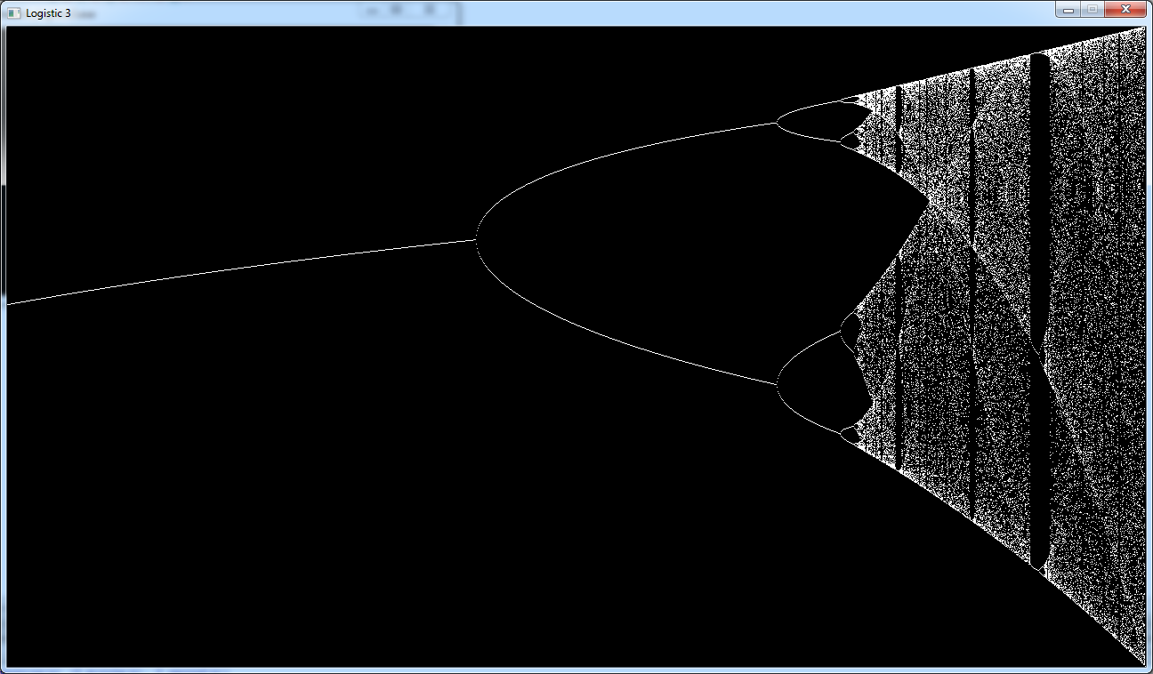
And here is the result

If you follow this diagram from left to right you can retrieve the observations we did before.

For low values of r there is only one stable point.
Then the line splits in 2 branches, when the population oscillates between 2 values
Then the 2 branches split into 4, and so on. Until quickly it becomes chaotic.

One interesting thing we can see is that the right part is not completely chaotic. There are some islands of
stability that can be explained when you look at the video about the Mandelbrot set.

This image looks like one we can see at the bottom of the wikipedia page although it is not the same model.
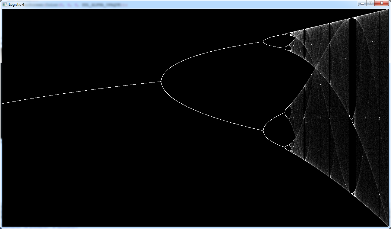
But above it some images looks nicer, and we can see more details in the chaotic zone.

The nicer diagram

When we look at these images we see that the pixels are not completely black or white there are various shades of
grey.
In fact these images shows several superimposed curves. We start with a blank background and each time we draw a
point we increase a little bit the R, G and B values of the pixel.

So this is what we will change in the code.
In the main loop, now we will draw 2000 points per column.

		for (int i = 0; i < 2000; i++)
		{

Then as before we compute the coordinates. But we need to tweak a little bit the value of r to avoid holes in the
branches.

			float r = startR + (endR - startR) * (t + (i % 10) / 10.0f) / (SCREEN_WIDTH - 1);
			float x = process(r, 10000 + i);
			float y = (1 - x) * (SCREEN_HEIGHT - 1);

Now instead of drawing a point, we will read the value of the pixel at these coordinates:

			Color col = gfx.getPixel(t, y);

Then we increase the values of the R, G and B components of this pixel, and we check if they don't go over 255:

			int c;

			c = col.r + 6;
			if (c > 255)
				c = 255;
			col.r = c;

			c = col.g + 6;
			if (c > 255)
				c = 255;
			col.g = c;

			c = col.b + 6;
			if (c > 255)
				c = 255;
			col.b = c;

And finally we write back the pixel to the screen.

			gfx.setPixel(t, y, col);
		}

		Download source code
		Download executable for Windows

And here is the resulting image: