The program in this article will need mouse input.
I modified System.cpp to handle the mouse events from SDL.
And I added these variables to the CSystem class:
		// mouse buttons
		#define BUT_LEFT    (1 << 0)
		#define BUT_RIGHT   (1 << 1)

		class CSystem
		{
		public:
			[...]

			Uint8   buttons;        // true while a button is pressed
			Uint8   buttonsDown;    // true only at the frame the button is pressed
			Uint8   buttonsUp;      // true only at the frame the button is released
			int     mouseX;
			int     mouseY;
mouseX an mouseY contains the mouse coordinates in pixels.
buttons, buttonsDown and buttonsUp are bit fields that contains 1 bit for each button.
The 2 buttons that are handled at the moment are BUT_LEFT and BUT_RIGHT respectively for the left and right
mouse buttons.
The bits in button are set to 1 while the corresponding button is pressed.
The bits in buttonsDown are set to 1 only during the frame the button is pressed.
The bits in buttonsUp are set to 1 only during the frame the button is released.
All these variables are updated in processEvents()
You'll see an example of how to use them in the program.
To handle the calculations on the polynomial, we will write a Polynomial class.
This class will store a polynomial of the form:
p(z) = c0*zn + c1*zn-1 + ... + cn-1*z + cn
Along with its roots.
So we will store a list of coefficients and a list of roots.
I use a std::vector which can be simply seen as an unlimited array, where you can add as many elements as you want.
		class Polynomial
		{
		private:
			std::vector<Complex> coefficients;

		public:
			std::vector<Complex> roots;
A degree() function will simply return the degree of the polynomial which is the number of its coefficients minus 1.
		int Polynomial::degree()
		{
			return coefficients.size() - 1;
		}
2 functions allows us to add a root or remove the last one.
		void Polynomial::addRoot(Complex r)
		{
			roots.push_back(r);
			coefficients.resize(roots.size() + 1);
		}

		void Polynomial::remRoot()
		{
			roots.pop_back();
			coefficients.resize(roots.size() + 1);
		}
A function allows us to evaluate the value of the polynomial for a given value of z.
Here we simply sum each power of z multiplied by its coefficient.
		Complex Polynomial::evaluate(Complex z)
		{
			Complex result = Complex(0, 0);
			Complex zn = Complex(1, 0);

			for (int i = degree(); i >= 0; i--)
			{
				result = result + zn * coefficients[i];
				zn = zn * z;
			}

			return result;
		}
The computation of the derivative is easy too.
We apply the classic derivation rule that says the derivative of z
n is n*z
n-1
		void Polynomial::derivative(Polynomial& result)
		{
			result.coefficients.clear();

			for (int i = 0; i <= degree()-1; i++)
			{
				Complex coef = coefficients[i] * (degree() - i);
				result.coefficients.push_back(coef);
			}
		}
The other function included in the Polynomial class is findCoefficients().
It is used to compute the polynomial coefficients from its roots.
As we saw before the polynomial has the form:
p(z) = c0*zn + c1*zn-1 + ... + cn-1*z + cn
When we know its roots, it can be written as a factorized form:
p(z) = (z - r0)(z - r1)...(z - rn-1)
If we expand this form we find that:
		c0 = 1
		c1 = (-r0) + (-r1) + ...
		c2 = (-r0)*(-r1) + (-r0)*(-r2) + ... + (-r1)*(-r2) + (-r1)*(-r3) + ...
		...
		cn = (-r0)*(-r1)*(-r2)...
Each coefficient c
m is the sum of all the combinations of m roots taken from all the roots.
To compute that we will need a list of indexes.
std::vector<int> idx;
Each of these indexes will represent a root number.
You can think of them as loop indexes.
To compute c
1, we will need 1 index that will go through roots r
0 to r
n-1.
For c
2, we will use 2 indexes each of which will point to a seperate root, to form each couple of roots we need to
add together.
But these indexes will follow some constraints.
First we don't want to count two times the same combination. For example we don't want both
(-r
0)*(-r
1) and (-r
1)*(-r
0).
The indexes must be all different too. We don't want (-r
0)*(-r
0).
To follow these rules we make sure that we always have:
idx[0] < idx[1] < ... < idx[n-1]
To follow that, at the beginning we will initialize them so that each one is equal to the previous one plus 1.
		idx[0] = 0;
		idx[1] = id[0] + 1;
		idx[2] = id[1] + 1;
		...
The indexes will not all go up to n-1 too. Because they must be all different, that implies that the last one will
go up to n-1, the previous one will only go up to n-2, the previous one will stop at n-3, and son on.
To increase these indexes we will begin at the last one.
We will add 1 to it. And if it goes over the number of roots, We consider the previous index.
We increase the previous index, and if it goes over the maximum, we continue to go up, until we reach an index that
doesn't overflow.
Then after increasing this index, we re-initialize the following ones with the rule we saw before.
Here is an example with 4 indexes and n roots.
At the beginning, we have:
		idx[0] = 0;
		idx[1] = 1;
		idx[2] = 2;
		idx[3] = 3;
We increase idx[3]. It now points to root number 4:
		idx[0] = 0;
		idx[1] = 1;
		idx[2] = 2;
		idx[3] = 4;
At the next step we increase it again.
		idx[0] = 0;
		idx[1] = 1;
		idx[2] = 2;
		idx[3] = 5;
And we go on until we reach n-1.
		idx[0] = 0;
		idx[1] = 1;
		idx[2] = 2;
		idx[3] = n-1;
Now if we increase it, it will be at n, that is over the number of roots.
		idx[0] = 0;
		idx[1] = 1;
		idx[2] = 2;
		idx[3] = n;
So we go up one level and we increase idx[2].
		idx[0] = 0;
		idx[1] = 1;
		idx[2] = 3;
		idx[3] = n;
Then we reinitialize idx[3] to idx[2] + 1:
		idx[0] = 0;
		idx[1] = 1;
		idx[2] = 3;
		idx[3] = 4;
And we can process this configuration.
Until we reach this state:
		idx[0] = 0;
		idx[1] = 1;
		idx[2] = n-2;
		idx[3] = n-1;
Now if we increase idx[3], it will again hit its maximum:
		idx[0] = 0;
		idx[1] = 1;
		idx[2] = n-2;
		idx[3] = n;
So we go up one level and increase idx[2], but it also reach its maximum which is n-1.
		idx[0] = 0;
		idx[1] = 1;
		idx[2] = n-1;
		idx[3] = n;
So we have to go up one step further and increase idx[1].
		idx[0] = 0;
		idx[1] = 2;
		idx[2] = n-1;
		idx[3] = n;
Then we can reinitialize idx[2] and idx[3] and go on with the process:
		idx[0] = 0;
		idx[1] = 2;
		idx[2] = 3;
		idx[3] = 4;
Implementation of findCoefficients
We already talked about the indexes list.
		void Polynomial::findCoefficients()
		{
			std::vector<int> idx;
			idx.resize(roots.size() + 1);
The first coefficient will always be 1.
coefficients[0] = 1;
Now we will loop to compute each of the other coefficients:
j is a handy variable that will be used as loop counter in various places.
			for (int i = 1; i <= degree(); i++)
			{
				coefficients[i] = Complex(0, 0);
				int j;
We initialize the indexes. Notice that the number of indexes we use depends on the number of the coefficient we are
calculating.
				for (j = 0; j < i; j++)
					idx[j] = j;
We start a loop were we will compute each term of the coefficient one after the other.
				while(true)
				{
We compute the term here by multyplying all of the roots we selected together.
					Complex c = Complex(1, 0);

					for (j = 0; j < i; j++)
						c = c * (-roots[idx[j]]);
And we add the term to the coefficient.
coefficients[i] = coefficients[i] + c;
Now we will increase the indexes following our rules to get to the next combination.
j will represent the current "level". At the beginning we point to the last index in our list.
j = i - 1;
We start a loop because we will perhabs get up several levels until we find an index that will not overflow.
					while(true)
					{
We try to increase the current index.
idx[j]++;
If this index reached its limit, we go up one level.
Unless we are already at the first index, in which case we break out of the loop.
						if (idx[j] == roots.size() - ((i-1) - j))
						{
							j--;
							if (j < 0)
								break;
						}
If we didn't reach a limit, this index was succesfully increased, then we re-initialize all the following indexes.
						else
						{
							for (int k = j + 1; k < i; k++)
								idx[k] = idx[k - 1] + 1;
							break;
						}
					}
If while moving up the levels we got before the first index, we break out of the loop. And we fall back to the
cefficients loop where we will compute the next coefficient.
					if (j < 0)
						break;
				}
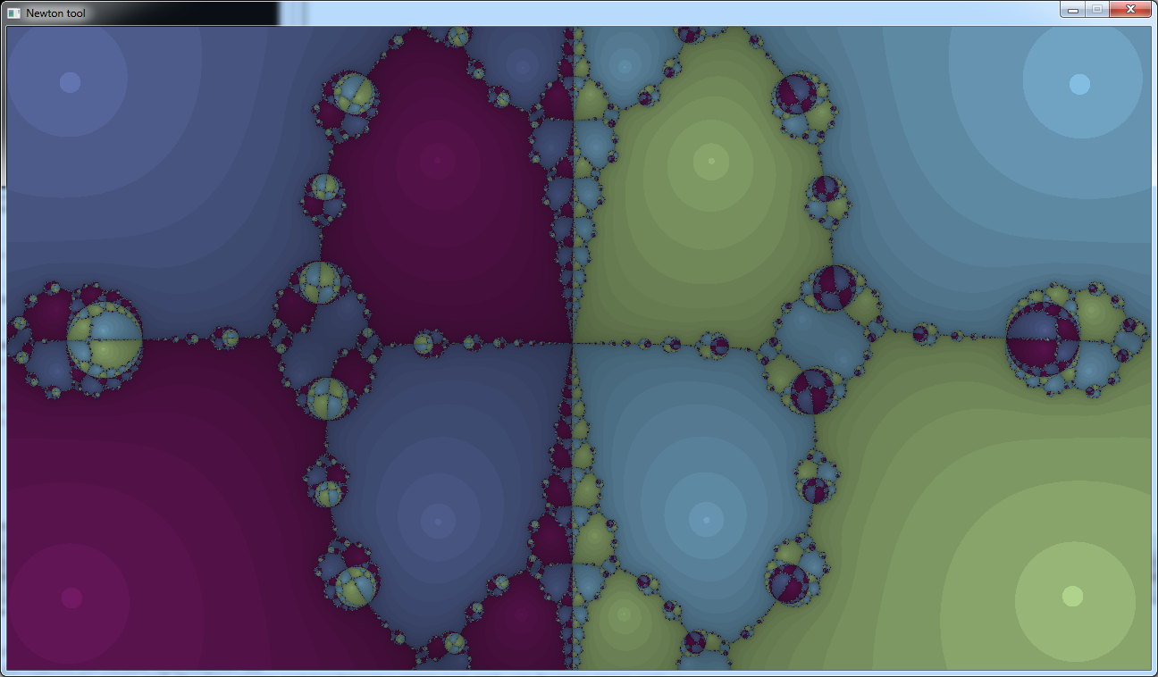
To be able to see the fractal drawing in real time, we will use a dithering pattern like I did for the
Mandelbrot.
The drawing function will only draw one point every 8 pixels along x and y:
		void drawNewton(int offsetX, int offsetY, std::vector<Color>& palette)
		{
			for (int yy = 0; yy < SCREEN_HEIGHT; yy += 8)
			{
				for (int xx = 0; xx < SCREEN_WIDTH; xx += 8)
				{
The rest of the function is the same as the drawing function we used in the
previous article.
Then in the main loop we will call this function with an x/y offset coming from a table to change the starting
point of the drawing.
		static Uint8 pattern[64] =
		{
			 0, 36,  4, 32, 18, 54, 22, 50,
			 2, 38,  6, 34, 16, 52, 20, 48,
			 9, 45, 13, 41, 27, 63, 31, 59,
			11, 47, 15, 43, 25, 61, 29, 57,
			 1, 37,  5, 33, 19, 55, 23, 51,
			 3, 39,  7, 35, 17, 53, 21, 49,
			 8, 44, 12, 40, 26, 62, 30, 58,
			10, 46, 14, 42, 24, 60, 28, 56
		};

		[...]

		while (sys.isQuitRequested() == false)
		{
			// draw the fractal
			if (frameCount < 64)
			{
				drawNewton(pattern[frameCount] % 8,
				           pattern[frameCount] / 8,
				           palette);
				frameCount++;
			}